An efficient tool to find multispecies MSY for interacting fish stocks

Disclaimer

The following vignette serves two main purposes. It is (i) a step-by-step introduction to the nash package, and (ii) a reproducible script where the code for the original article https://doi.org/10.1111/faf.12817 is archived.

Benchmark Models

In the original Fish and Fisheries article, the nash package was applied to three models of distinct complexity with regards to the number of species ( $S$ ) within the stock-complex for which $\mathbf{F}_\textbf{Nash}$ is computed. These are, (i) Taylor and Crizer (2005) modified two-species competitive Lotka-Volterra (LV) model; and (ii) ICES (2017) Baltic Sea and (iii) ICES (2016) North Sea Ecopath with Ecosim (Christensen and Walters 2004; Steenbeek et al. 2016) models, both of which were ported into R using the Rpath https://github.com/NOAA-EDAB/Rpath (Aydin, Lucey, and Gaichas 2016; Lucey, Gaichas, and Aydin 2020).

Complexity increases with respect to the number of interacting species and trophic links modelled; from $2$ species and $2$ links for the modified LV model to $22$ and $69$ compartments and $82$ and $968$ links for the Baltic Sea and North Sea models, respectively. The following snapshots represent these latter two EwE models showcasing as non-grey nodes the $S$ species with commercial value whose harvesting rates we optimised, whilst capturing its effect on the entire food web.

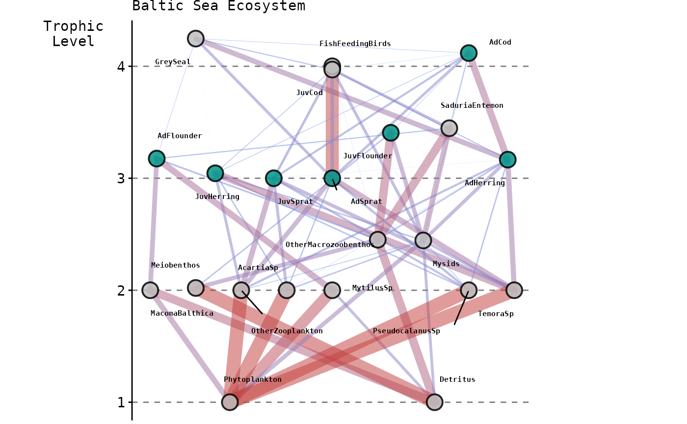
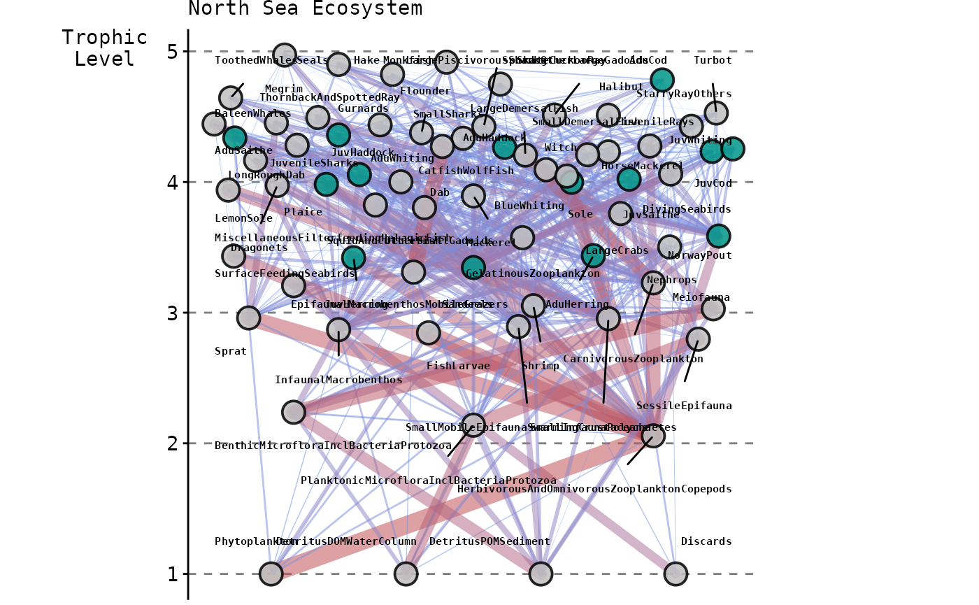
It is important to note that both the Baltic and North Sea models are used as ‘key-run’ parameterisations peer-reviewed by the Working Group on Multispecies Assessment Methods (WGSAM) to inform management advice provided by the International Council for the Exploration of the Sea (ICES).

Running `nash` with `Rpath` models

To support users employing Rpath as their operating model, a built-in function fn_rpath has been included within the nash package to provide the input function fn. The function is capable of transparently handling models in which all or some of the exploited compartments are stage structured (e.g. all species in the Baltic Sea model and Cod, Whiting, Haddock, Saithe and Herring in the North Sea model).

### NOT EVALUATING THIS CHUNK GIVEN THE RUNNING TIME NEEDED TO FIND NE FOR  ###
###   COMPLEX ECOLOGICAL MODELS. IT IS POSSIBLE TO REPRODUCE THE RESULTS BY ###
###   COPY/PASTING IN YOUR LOCAL MACHINE.                                   ###
# Load libraries
library(nash)
library(Rpath)
# Load the BS model
load("BalticSeaModel.RData")
# Commercial stock-complex
spp = c("AdCod", "AdHerring", "AdSprat", "AdFlounder")
# Initialising search with last year of data Fs
par <- as.numeric(tail(Rsim.model$fishing$ForcedFRate[, spp], n = 1))
# Running nash via LV
nash.eq.LV.BS <- nash(
  par = par,
  fn = fn_rpath,
  aged.str = TRUE,
  data.years = 10,
  rsim.mod = Rsim.model,
  IDnames = c(
    "JuvCod",
    "AdCod",
    "JuvHerring",
    "AdHerring",
    "JuvSprat",
    "AdSprat",
    "JuvFlounder",
    "AdFlounder"
  ),
  method = "LV",
  yield.curves = TRUE,
  rpath.params = Rpath.parameters,
  avg.window = 250,
  simul.years = 500,
  integration.method = "AB",
  conv.criterion = 0.01,
  F.increase = 0.01
)
# Load the NS model
load("NorthSeaModel.RData")
# Commercial stock-complex
spp = c(
  "AduCod",
  "AduWhiting",
  "AduHaddock",
  "AduSaithe",
  "AduHerring",
  "NorwayPout",
  "Sandeels",
  "Plaice",
  "Sole"
)
# Initialising search with last year of data Fs
par <- Rsim.model$fishing$ForcedFRate[sim.years, spp]
# Running nash via LV
nash.eq.LV.NS <- nash(
  par = par,
  fn = fn_rpath,
  aged.str = TRUE,
  data.years = 23,
  rsim.mod = Rsim.model,
  IDnames = c(
    "JuvCod",
    "AduCod",
    "JuvWhiting",
    "AduWhiting",
    "JuvHaddock",
    "AduHaddock",
    "JuvSaithe",
    "AduSaithe",
    "JuvHerring",
    "AduHerring",
    "NorwayPout",
    "Sandeels",
    "Plaice",
    "Sole"
  ),
  method = "LV",
  yield.curves = TRUE,
  rpath.params = Rpath.parameters,
  avg.window = 500,
  simul.years = 1000,
  integration.method = "AB",
  conv.criterion = 0.01
)

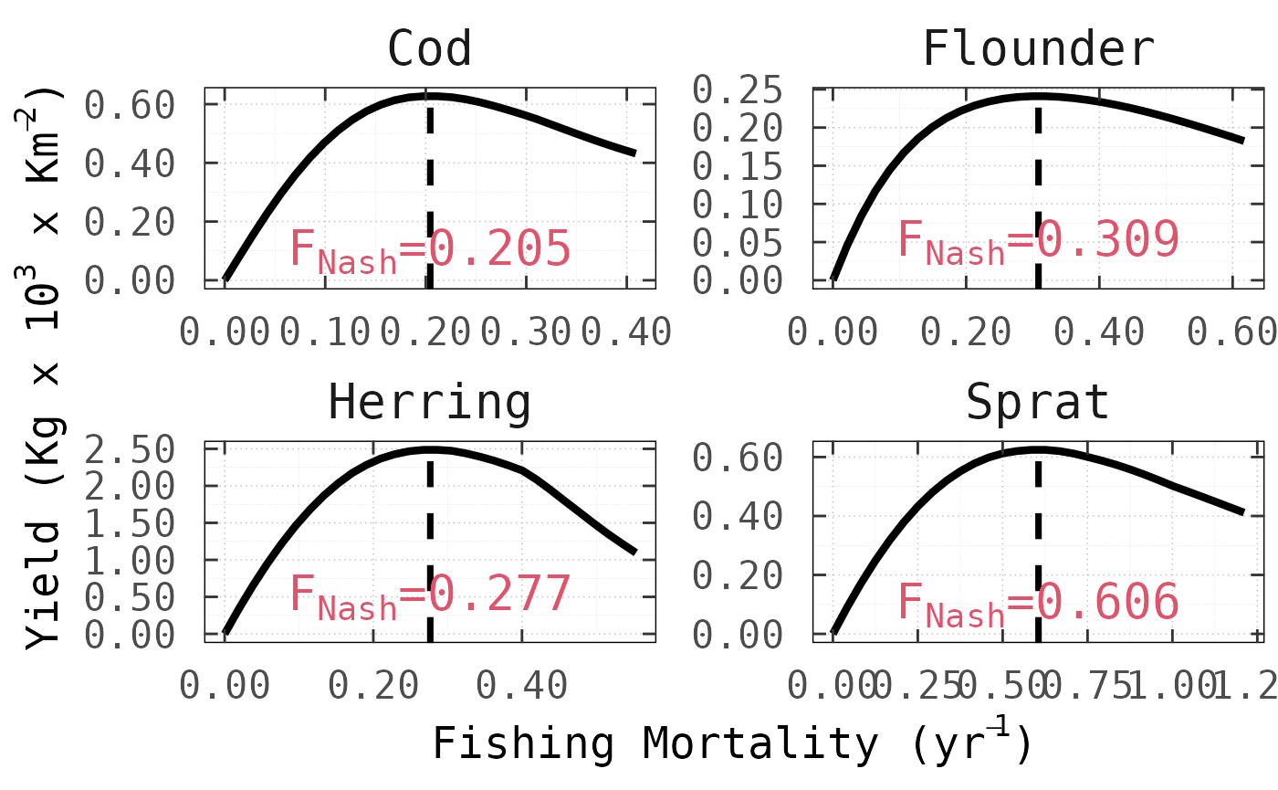
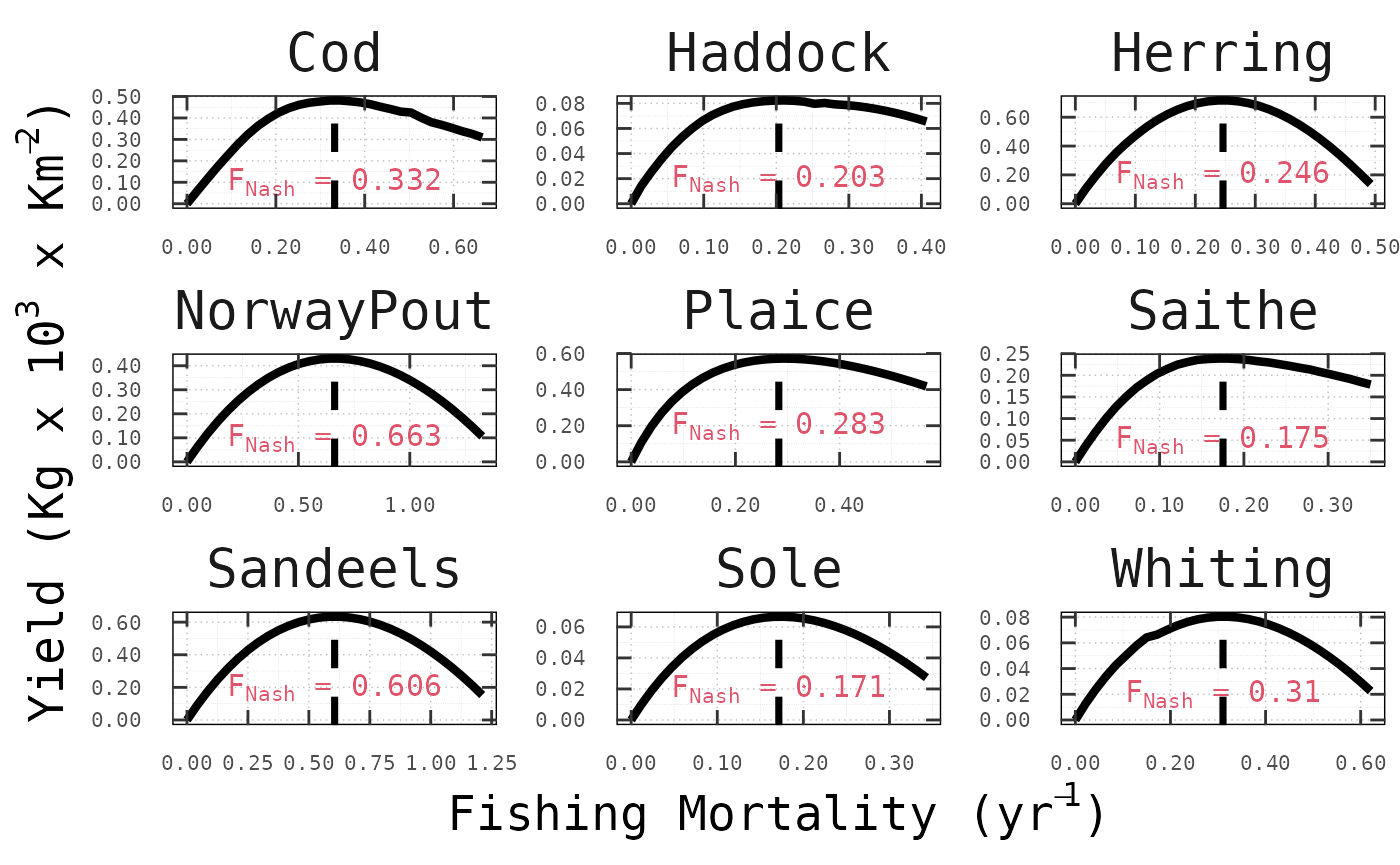
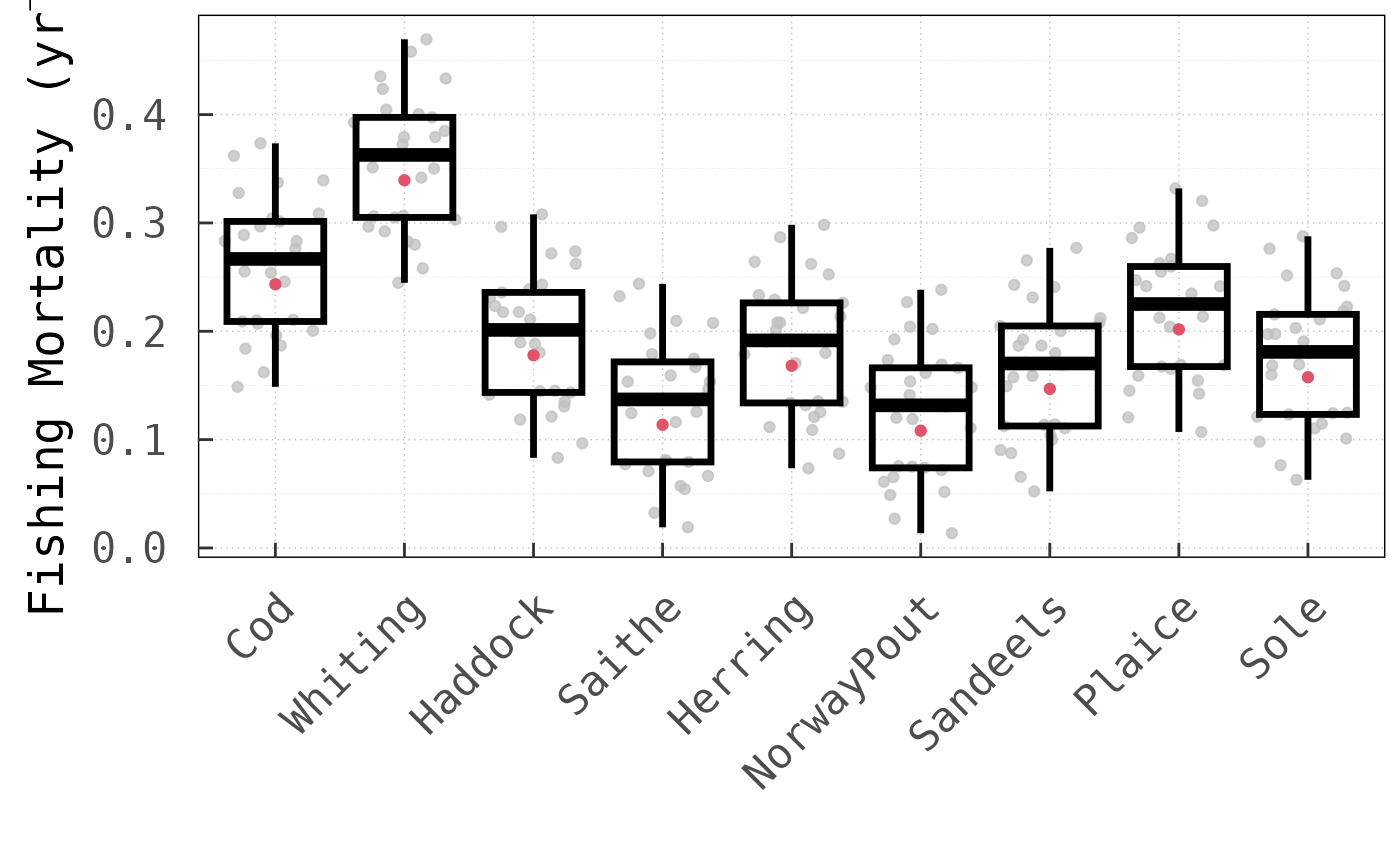
Once executed, it is possible to test whether NE-MSY has been achieved by varying the fishing mortality on each stock in turn while keeping the others fixed at $\mathbf{F}_\textbf{Nash}$ . This is precisely what the following figures show for all $S$ species and across models, where nash correctly computed the Nash equilibrium fishing mortality rates (vertical dashed lines), such that, for no stock the long-term yeld can be increased by choosing a different fishing mortality.

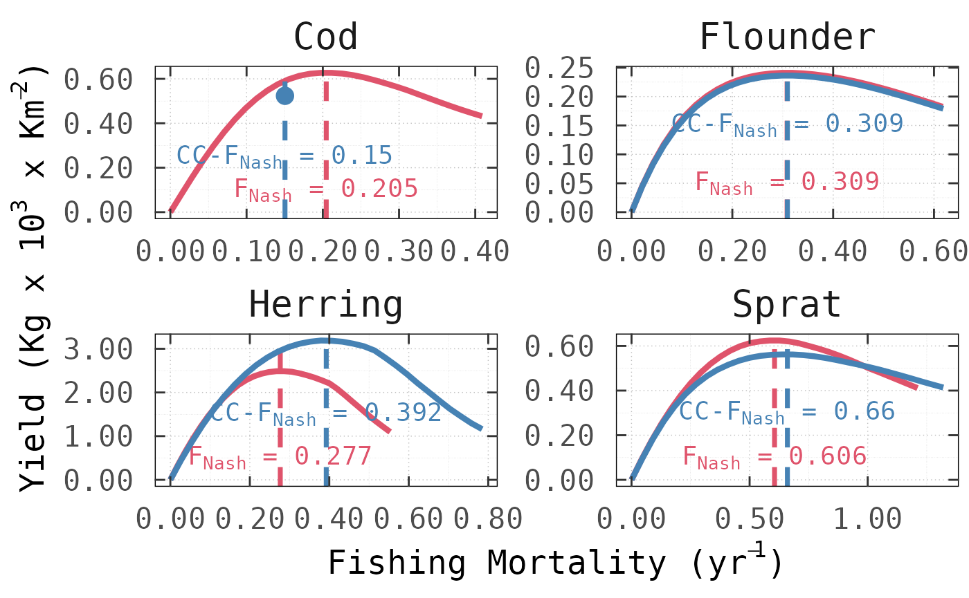
Applying `nash` with Conservation Constraints

It is conceivable that in some cases harvesting at the Nash equilibrium might drive one or more species to extinction. Even if this does not happen, some species might be placed under unacceptable risk levels of stock collapse. Therefore, the nash package includes an option that allows the user to explicitly incorporate conservation constraints (Matsuda and Abrams 2006), specifying a conservation biomass threshold Bcons below which stock sizes are not permitted to fall.

We showcase this functionality with the Baltic Sea ecosystem by adding a conservation constraint for the biomass of Cod; which we chose arbitrarily by holding Cod $1 \times 10^5 \text{ Tn}$ above the original $B_{\text{Nash,Cod}}$ (i.e. $\approx 84 \times 10^4 \text{ Tn}$ ).

# Load the BS model and reference Nash equilibrium results
load("Data/BalticSeaModel.RData")
nash.eq.LV.BS <- readRDS("BS-NE-Fmsy-LV.rds")
# Commercial stock-complex
spp = c("AdCod", "AdHerring", "AdSprat", "AdFlounder")
# Initialising search with last year of data Fs
par <- as.numeric(tail(Rsim.model$fishing$ForcedFRate[, spp], n = 1))
# Baltic Sea Modelled Area
model.area <- 240669
# Target for Cod biomass = 1e5 (kg^3)
blim <-
  c((
    as.numeric(nash.eq.LV.BS$value / nash.eq.LV.BS$par)[1] + (100000 / model.area)
  ), 0, 0, 0)
# Running nash via LV
nash.eq.LV.BS.CC <- nash(
  par = par,
  fn = fn_rpath,
  aged.str = TRUE,
  data.years = 10,
  rsim.mod = Rsim.model,
  IDnames = c(
    "JuvCod",
    "AdCod",
    "JuvHerring",
    "AdHerring",
    "JuvSprat",
    "AdSprat",
    "JuvFlounder",
    "AdFlounder"
  ),
  method = "LV",
  yield.curves = FALSE,
  rpath.params = Rpath.parameters,
  avg.window = 250,
  simul.years = sim.years,
  integration.method = "RK4",
  Bcons = blim,
  track = TRUE,
  conv.criterion = 0.01
)

This results in a new set of $\mathbf{F_{Nash}}$ values in which, as expected, the fishing pressure on Cod needs to be tapered from $0.204 \text{ year}^{−1}$ to $0.150 \text{ year}^{−1}$ with its consequent reduction in yield from $\approx 15 \times 10^4 \text{ Tn year}^{−1}$ to $\approx 13 \times 10^4 \text{ Tn year}^{−1}$ . Application of the constraint increased $F_{\text{Nash,Herring}}$ from $0.277 \text{ year}^{−1}$ to $0.392 \text{ year}^{−1}$ generating a surplus of $\approx 17 \times 10^4 \text{ Tn year}^{−1}$ but had little influence on the NE-MSY harvesting rates for Flounder. For Sprat, by contrast, the conservation constraint on Cod led to a higher $F_{\text{Nash,Sprat}}$ of $0.660 \text{ year}^{−1}$ with a marginal reduction in yield of $\approx 1 \times 10^3 \text{ Tn year}^{−1}$ .

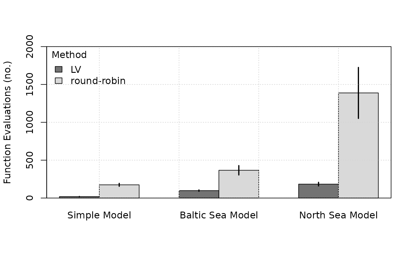
`nash`’s `LV` algorithm vs `round-robin`

A key advantage of the LV method over the simple round-robin method, that is, sequential optimisation of each $F_i$ until convergence is reached, is that it requires much less computation time, especially for complex ecological communities. As a platform-independent metric of performance, we compared the number of objective function evaluations between the two methods. For this analysis, we applied both methods across the three tested models with $n=77$ different initial harvesting rate values.

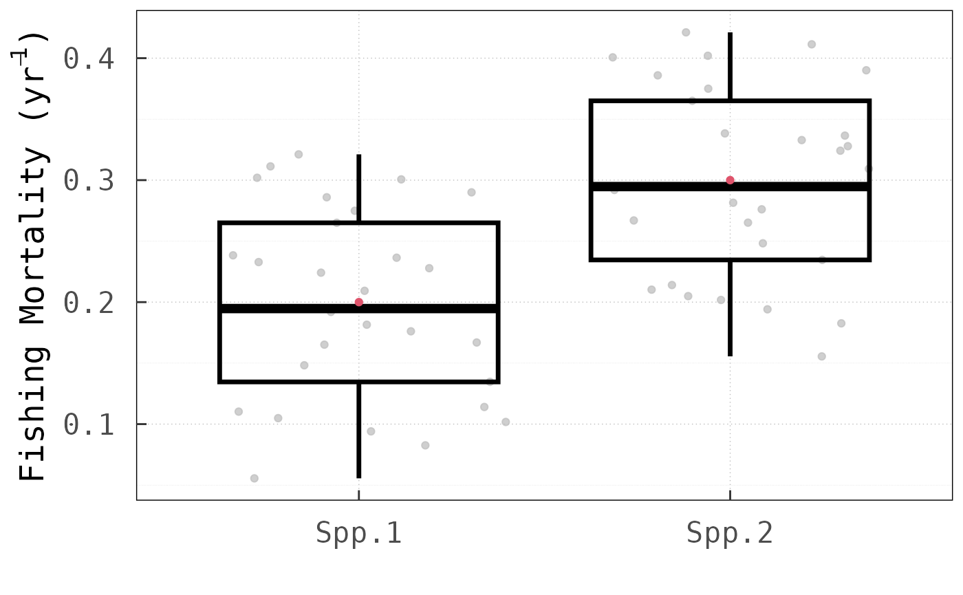
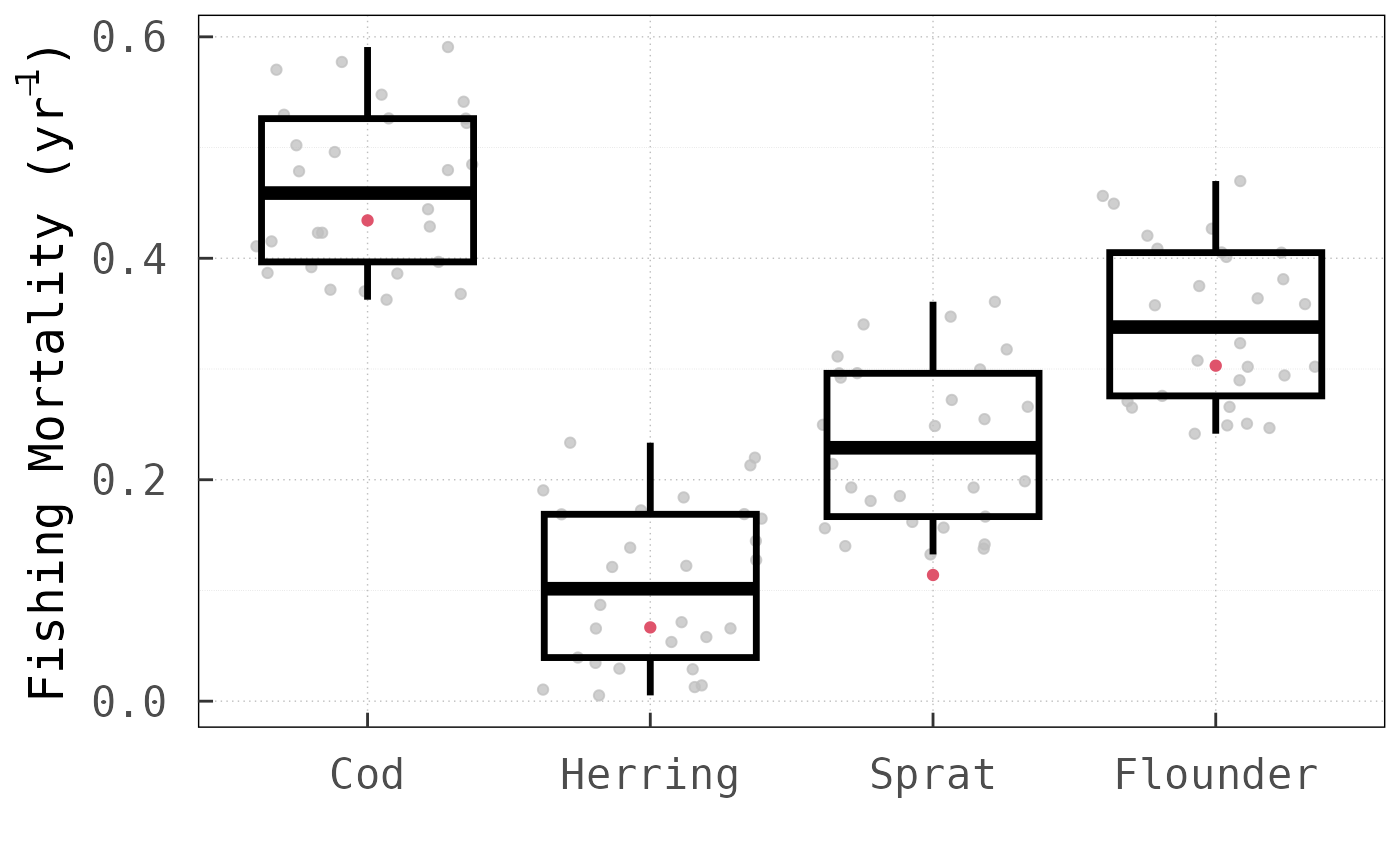
In all cases, the LV method outperformed the round-robin method for the same convergence threshold (set to a value of $0.01$ for this analysis). Noteworthy is, in particular, that for the North Sea model, the LV method requires only $1.88$ times more function evaluations than for the Baltic Sea model, even though the dimension of the $\mathbf{F}_\textbf{Nash}$ vector increases by $2.25$ from $4$ to $9$ . Using the round-robin method, by comparison, the number of function evaluations increases $7$ -fold.

References

Aydin, Kerim, Sean Lucey, and Sarah Gaichas. 2016. Rpath: R Implementation of Ecopath with Ecosim. https://github.com/NOAA-EDAB/Rpath.

Christensen, Villy, and Carl J Walters. 2004. “Ecopath with Ecosim: Methods, Capabilities and Limitations.” Ecological Modelling 172 (2): 109–39. https://doi.org/https://doi.org/10.1016/j.ecolmodel.2003.09.003.

ICES. 2016. “Report of the Working Group on Multispecies Assessment Methods (WGSAM), 9-13 November 2015, Woods Hole, USA.” ICES CM 2015/SSGEPI:20.

———. 2017. “Report of the Working Group on Multispecies Assessment Methods (WGSAM), 10–14 October 2016, Reykjavik, Iceland.” ICES CM 2016/SSGEPI:21, 1–94. https://doi.org/https://doi.org/10.17895/ices.pub.8534.

Lucey, Sean M., Sarah K. Gaichas, and Kerim Y. Aydin. 2020. “Conducting Reproducible Ecosystem Modeling Using the Open Source Mass Balance Model Rpath.” Ecological Modelling 427: 109057. https://doi.org/https://doi.org/10.1016/j.ecolmodel.2020.109057.

Matsuda, Hiroyuki, and Peter A. Abrams. 2006. “Maximal Yields from Multispecies Fisheries Systems: Rules for Systems with Multiple Trophic Levels.” Ecological Applications 16 (1): 225–37. https://doi.org/https://doi.org/10.1890/05-0346.

Steenbeek, Jeroen, Joe Buszowski, Villy Christensen, Ekin Akoglu, Kerim Aydin, Nick Ellis, Dalai Felinto, et al. 2016. “Ecopath with Ecosim as a Model-Building Toolbox: Source Code Capabilities, Extensions, and Variations.” Ecological Modelling 319: 178–89. https://doi.org/https://doi.org/10.1016/j.ecolmodel.2015.06.031.

Taylor, Austin, and Amy Crizer. 2005. “A Modified Lotka-Volterra Competition Model with a Non-Linear Relationship Between Species.” Rose-Hulman Undergraduate Mathematics Journal 6 (2). https://scholar.rose-hulman.edu/rhumj/vol6/iss2/8.

Disclaimer

Benchmark Models

Running nash with Rpath models

Applying nash with Conservation Constraints

nash’s LV algorithm vs round-robin

References

Running `nash` with `Rpath` models

Applying `nash` with Conservation Constraints

`nash`’s `LV` algorithm vs `round-robin`